SIOP 2018: An Analysis of Tweets Using Natural Language Processing with Topic Modeling

Challenge 1: Getting the Data into R

To get data from Twitter into R, you need to log into Twitter and create an app. This is easier than it sounds.

1. Log into Twitter.
2. Go to http://apps.twitter.com and click Create New App.
3. Complete the form and name your app whatever you want. I named mine rnlanders R Interface.
4. Once you have created your app, open its settings and navigate to Keys and Access Tokens.
5. Copy-paste the four keys you see into the block of code below.

# Replace these with your Twitter access keys - DO NOT SHARE YOUR KEYS WITH OTHERS
consumer_key <- "xxxxxxxxxxxx"
consumer_secret <- "xxxxxxxxxxxxxxxxxxxxxxxx"
access_token <- "xxxxxxxxxxxxxxxxxxxxxxxx"
access_token_secret <- "xxxxxxxxxxxxxxxxxxxxxxxx"

# Now, authorize R to use Twitter using those keys
# Remember to select "1" to answer "Yes" to the question about caching.
setup_twitter_oauth(consumer_key, consumer_secret, access_token, access_token_secret)

Finally, we need to actually download all of those data. This is really two steps: download tweets as a list, then convert the list into a data frame. We’ll just grab the most recent 2000, but you could grab all of them if you wanted to.

twitter_list <- searchTwitter("#siop18", n=2000)
twitter_tbl <- as.tibble(twListToDF(twitter_list))

Challenge 2: Pre-process the tweets, convert into a corpus, then into a dataset

That text is pretty messy – there’s a lot of noise and nonsense in there. If you take a look at a few tweets in twitter_tbl, you’ll see the problem yourself. To deal with this, you need to pre-process. I would normally do this in a tidyverse magrittr pipe but will write it all out to make it a smidge clearer (although much longer).

Importantly, this won’t get everything. There is a lot more pre-processing you could do to get this dataset even cleaner, if you were going to use this for something other than a blog post! But this will get you most of the way there, and close enough that the analysis we’re going to do afterward won’t be affected.

# Isolate the tweet text as a vector
tweets <- twitter_tbl$text
# Get rid of retweets
tweets <- tweets[str_sub(tweets,1,2)!="RT"]
# Strip out clearly non-English characters (emoji, pictographic language characters)
tweets <- str_replace_all(tweets, "\\p{So}|\\p{Cn}", "")
# Convert to ASCII, which removes other non-English characters
tweets <- iconv(tweets, "UTF-8", "ASCII", sub="")
# Strip out links
tweets <- str_replace_all(tweets, "http[[:alnum:][:punct:]]*", "")
# Everything to lower case
tweets <- str_to_lower(tweets)
# Strip out hashtags and at-mentions
tweets <- str_replace_all(tweets, "[@#][:alnum:]*", "")
# Strip out numbers and punctuation and whitespace
tweets <- stripWhitespace(removePunctuation(removeNumbers(tweets)))
# Strip out stopwords 
tweets <- removeWords(tweets, stopwords("en"))
# Stem words
tweets <- stemDocument(tweets)
# Convert to corpus
tweets_corpus <- Corpus(VectorSource(tweets))
# Convert to document-term matrix (dataset)
tweets_dtm <- DocumentTermMatrix(tweets_corpus)
# Get rid of relatively unusual terms
tweets_dtm <- removeSparseTerms(tweets_dtm, 0.99)

Challenge 3: Get a general sense of topics based upon word counts alone

Now that we have a dataset, let’s do a basic wordcloud visualization. I would recommend against trying to interpret this too closely, but it’s useful to double-check that we didn’t miss anything (e.g., if there was a huge “ASDFKLAS” in this word cloud, it would be a signal that I did something wrong in pre-processing). It’s also great coffee-table conversation?

# Create wordcloud
wordCounts <- colSums(as.tibble(as.matrix(tweets_dtm)))
wordNames <- names(as.tibble(as.matrix(tweets_dtm)))
wordcloud(wordNames, wordCounts, max.words=75)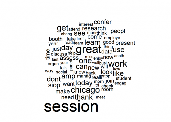

# We might also just want a table of frequent words, so here's a quick way to do that
tibble(wordNames, wordCounts) %>% arrange(desc(wordCounts)) %>% top_n(20)

## # A tibble: 20 x 2
##    wordNames wordCounts
##    <chr>          <dbl>
##  1 session          115
##  2 great             75
##  3 work              56
##  4 chicago           51
##  5 get               49
##  6 one               46
##  7 day               43
##  8 can               43
##  9 like              42
## 10 thank             42
## 11 use               42
## 12 learn             42
## 13 dont              41
## 14 amp               41
## 15 today             40
## 16 see               40
## 17 siop              37
## 18 look              36
## 19 confer            35
## 20 new               34

These stems reveal what you’d expect: most people talking about #siop18 are talking about conference activities themselves – going to sessions, being in Chicago, being part of SIOP, looking around seeing things, etc. A few stick out, like thank and learn.

Of course, this is a bit of an exercise in tea-leaves reading, and there’s a huge amount of noise since people pick particular words to express themselves for a huge variety of reasons. So let’s push a bit further. We want to know if patterns emerge within these words surrounding latent topics.

Challenge 4: Let’s see if we can statistically extract some topics and interpret them

For this final analytic step, we’re going to run latent Dirichlet allocation (LDA) and see if we can identify some latent topics. The dataset is relatively small as far as LDA goes, but perhaps we’ll get something interesting out of it!

First, let’s see how many topics would be ideal to extract using ldatuning. I find it useful to do two of these in sequence, to get the “big picture” and then see where a precise cutoff might be best.

# First, get rid of any blank rows in the final dtm
final_dtm <- tweets_dtm[unique(tweets_dtm$i),]
# Next, run the topic analysis and generate a visualization
topic_analysis <- FindTopicsNumber(final_dtm, 
                                   topics = seq(2,100,5), 
                                   metrics=c("Griffiths2004","CaoJuan2009","Arun2010","Deveaud2014"))
FindTopicsNumber_plot(topic_analysis)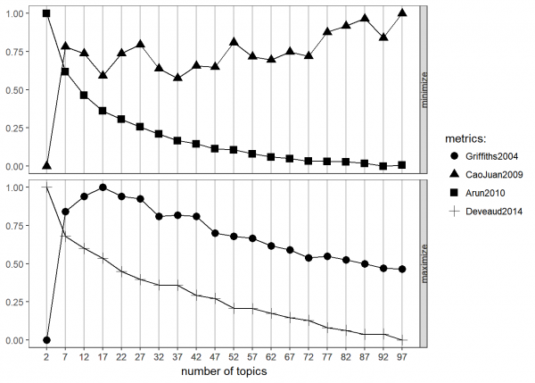

The goal of this analysis is to find the point at which the various metrics (or the one you trust the most) is either minimized (in the case of the top two metrics) or maximized (in the case of the bottom two). It is conceptually similar to interpreting a scree plot for factor analysis.

As is pretty common in topic modeling, there’s no great answer here. Griffiths suggests between 10 and 25 somewhere, Cao & Juan suggests the same general range although noisier, Arun is not informative, nor is Deveaud. This could be the result of poor pre-processing (likely contributes, since we didn’t put a whole lot of effort into spot-checking the dataset to clean it up completely!) or insufficient sample size (also likely) or just a noisy dataset without much consistency. Given these results, let’s zoom in on 10 to 25 with the two approaches that seem to be most helpful.

topic_analysis <- FindTopicsNumber(final_dtm, 
                                   topics = seq(10,26,2), 
                                   metrics=c("Griffiths2004","CaoJuan2009"))
FindTopicsNumber_plot(topic_analysis)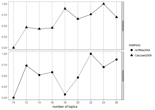

These are both very noisy, but I’m going to go with 18. In real-life modeling, you would probably want to try values throughout this range and try to interpret what you find within each.

Now let’s actually run the final LDA. Note that in a “real” approach, we might use a within-sample cross-validation approach to develop this model, but here, we’re prioritizing demonstration speed.

# First, conduct the LDA
tweets_lda <- LDA(final_dtm, k=18)

# Finally, list the five most common terms in each topic
tweets_terms <- as.data.frame(tweets_lda@beta)  %>% # grab beta matrix
  t %>%           # transpose so that words are rows
  as.tibble %>%   # convert to tibble (tidyverse data frame)
  bind_cols(term = tweets_lda@terms)  # add the term list as a variable
names(tweets_terms) <- c(1:18,"term") # rename them to numbers

# Visualize top term frequencies
tweets_terms %>%
  gather(key="topic",value="beta",-term,convert=T) %>%
  group_by(topic) %>%
  top_n(10, beta) %>%
  select(topic, term, beta) %>%
  arrange(topic,-beta) %>%
  print(n = Inf)

## # A tibble: 180 x 3
## # Groups:   topic [18]
##     topic term      beta
##     <int> <chr>    <dbl>
##   1     1 chicago  -1.32
##   2     1 confer   -1.98
##   3     1 home     -2.70
##   4     1 bring    -3.07
##   5     1 day      -3.28
##   6     1 back     -3.79
##   7     1 siop     -3.97
##   8     1 work     -4.01
##   9     1 time     -4.03
##  10     1 morn     -4.22
##  11     2 research -2.80
##  12     2 session  -3.27
##  13     2 can      -3.40
##  14     2 need     -3.45
##  15     2 work     -3.51
##  16     2 team     -3.65
##  17     2 booth    -3.79
##  18     2 get      -3.82
##  19     2 come     -3.94
##  20     2 your     -3.94
##  21     3 can      -3.12
##  22     3 differ   -3.26
##  23     3 get      -3.37
##  24     3 dont     -3.44
##  25     3 your     -3.46
##  26     3 great    -3.47
##  27     3 good     -3.51
##  28     3 today    -3.63
##  29     3 see      -3.75
##  30     3 organ    -3.80
##  31     4 great    -2.70
##  32     4 session  -2.78
##  33     4 year     -3.45
##  34     4 siop     -3.61
##  35     4 see      -3.63
##  36     4 work     -3.63
##  37     4 amp      -3.67
##  38     4 take     -3.72
##  39     4 morn     -3.73
##  40     4 mani     -3.83
##  41     5 session  -2.37
##  42     5 one      -2.79
##  43     5 can      -3.14
##  44     5 work     -3.50
##  45     5 manag    -3.69
##  46     5 amp      -3.92
##  47     5 peopl    -3.92
##  48     5 day      -3.96
##  49     5 great    -4.00
##  50     5 develop  -4.05
##  51     6 cant     -2.96
##  52     6 one      -2.96
##  53     6 say      -3.03
##  54     6 wait     -3.10
##  55     6 now      -3.40
##  56     6 today    -3.52
##  57     6 learn    -3.53
##  58     6 data     -3.66
##  59     6 can      -3.69
##  60     6 let      -3.71
##  61     7 social   -2.40
##  62     7 great    -3.05
##  63     7 know     -3.36
##  64     7 assess   -3.50
##  65     7 session  -3.51
##  66     7 now      -3.61
##  67     7 will     -3.62
##  68     7 job      -3.72
##  69     7 use      -3.80
##  70     7 back     -3.84
##  71     8 session  -2.07
##  72     8 great    -2.84
##  73     8 learn    -2.99
##  74     8 like     -3.08
##  75     8 research -3.35
##  76     8 look     -3.81
##  77     8 work     -4.04
##  78     8 peopl    -4.09
##  79     8 today    -4.10
##  80     8 still    -4.19
##  81     9 like     -2.99
##  82     9 day      -3.06
##  83     9 way      -3.31
##  84     9 tri      -3.39
##  85     9 room     -3.44
##  86     9 session  -3.62
##  87     9 think    -3.70
##  88     9 want     -3.84
##  89     9 booth    -3.87
##  90     9 know     -3.88
##  91    10 take     -2.69
##  92    10 good     -3.15
##  93    10 dont     -3.20
##  94    10 game     -3.27
##  95    10 siop     -3.36
##  96    10 analyt   -3.48
##  97    10 need     -3.51
##  98    10 research -3.51
##  99    10 look     -3.57
## 100    10 new      -3.64
## 101    11 work     -2.92
## 102    11 engag    -3.15
## 103    11 session  -3.27
## 104    11 learn    -3.37
## 105    11 can      -3.61
## 106    11 great    -3.67
## 107    11 employe  -3.69
## 108    11 amp      -3.73
## 109    11 get      -3.79
## 110    11 year     -3.90
## 111    12 use      -2.37
## 112    12 question -3.16
## 113    12 one      -3.24
## 114    12 twitter  -3.26
## 115    12 busi     -3.30
## 116    12 thing    -3.35
## 117    12 leader   -3.36
## 118    12 day      -3.56
## 119    12 data     -3.65
## 120    12 learn    -3.79
## 121    13 student  -3.21
## 122    13 work     -3.24
## 123    13 present  -3.34
## 124    13 look     -3.43
## 125    13 new      -3.48
## 126    13 employe  -3.54
## 127    13 see      -3.81
## 128    13 want     -3.83
## 129    13 make     -3.86
## 130    13 organ    -4.00
## 131    14 committe -2.97
## 132    14 like     -3.34
## 133    14 come     -3.45
## 134    14 join     -3.46
## 135    14 thank    -3.53
## 136    14 discuss  -3.54
## 137    14 work     -3.58
## 138    14 now      -3.58
## 139    14 present  -3.62
## 140    14 dont     -3.66
## 141    15 great    -2.56
## 142    15 session  -2.59
## 143    15 thank    -3.10
## 144    15 like     -3.26
## 145    15 new      -3.39
## 146    15 today    -3.49
## 147    15 employe  -3.70
## 148    15 booth    -3.86
## 149    15 back     -3.87
## 150    15 dont     -3.91
## 151    16 see      -2.65
## 152    16 thank    -3.17
## 153    16 focus    -3.19
## 154    16 siop     -3.20
## 155    16 session  -3.31
## 156    16 help     -3.56
## 157    16 get      -3.56
## 158    16 amp      -3.58
## 159    16 assess   -3.76
## 160    16 work     -3.82
## 161    17 get      -2.60
## 162    17 day      -3.05
## 163    17 today    -3.30
## 164    17 field    -3.34
## 165    17 come     -3.65
## 166    17 last     -3.66
## 167    17 learn    -3.86
## 168    17 peopl    -3.95
## 169    17 phd      -3.96
## 170    17 good     -3.97
## 171    18 session  -2.98
## 172    18 realli   -3.24
## 173    18 thank    -3.24
## 174    18 poster   -3.29
## 175    18 time     -3.41
## 176    18 think    -3.65
## 177    18 look     -3.66
## 178    18 best     -3.68
## 179    18 present  -3.77
## 180    18 talk     -3.79

There’s a bit of tea-leaves-reading here again, but now instead of trying to interpret individual items, we are trying to identify emergent themes, similar to what we might do with an exploratory factor analysis.

For example, we might conclude something like:

• Theme 1 seems related to travel back from the conference (chicago, conference, home, back, time).
• Theme 2 seems related to organizational presentations of research (research, work, team, booth).
• Theme 7 seems related to what people will bring back to their jobs (social, assess, use, job, back).
• Theme 9 seems related to physical locations (room, session, booth).
• Theme 11 seems related to learning about employee engagement (work, engage, session, learn, employee).
• Theme 14 seems related to explaining SIOP committee work (committee, like, join, thank, discuss, present).

And so on.

At this point, we would probably want to dive back into the dataset to check out interpretations against the tweets that were most representative of their categories. We might even cut out a few high-frequency words (like “work” or “thank” or “poster”) because they may be muddling the topics due to their high frequencies. Many options. But it is important to treat it as a process of iterative refinement. No quick answers here; human interpretation is still central.

In any case, that’s quite enough detail for a blog post! So I’m going to cut if off there.

I hope that despite the relatively rough approach taken here, this has demonstrated to you the complexity, flexibility, and potential value of NLP and topic modeling for interpreting unstructured text data. It is an area you will definitely want to investigate for your own organization or research.