Translating the Words Used in Machine Learning into Human Language

When trying to learn about machine learning, one of the biggest initial hurdles for social scientists, or even traditional statisticians, are the differences in terminology. The gap between the way social scientists talk about statistical concepts and the way machine learning experts talk about the same concepts is so vast that many social scientists do not even realize that they are running statistical analyses that involve machine learning! You may be using machine learning and not even realize it! So here’s a glossary to convert words you see into machine learning into words you already know.

Importantly, I’ve written these in an order where the build on each other.  So you might start reading from the top and then just stop whenever it’s gone over your head… because it’s just going to get worse!

• algorithm: Any carefully defined step by step process that converts inputs into outputs.  When you run an ANOVA in SPSS, you convert raw data (input) into an ANOVA table (output).  Thus, you have executed an ANOVA algorithm.  When you calculate a mean on pencil and paper by adding numbers together (step 1) and then dividing by the number of items (step 2), you have also executed an algorithm.
• learning: Fundamentally, the term “learning” in this context just refers to any procedure that allow you to make predictions about new data given current data.  For example, 1-predictor univariate ordinary least squares (OLS) regression allows you to make predictions of y given x.  Thus, OLS regression is a learning algorithm.  Factor analysis allows you to make predictions of latent categories among your variables.  Thus, factor analysis is also a learning algorithm.
• statistical learning algorithm: Any statistical procedure that you already know how to do involves a statistical learning algorithm; it enables you to make population predictions from given data by solving a step-by-step mathematical manipulation of a dataset.  Regression, factor analysis, cluster analysis, and ANOVA all involve statistical learning.
• supervised learning: A learning algorithm with a known DV.  Examples of supervised statistical learning algorithms are OLS regression and ANOVA using the formulas you already know.
• unsupervised learning: A learning algorithm without a known DV.  Examples of unsupervised statistical learning algorithms are exploratory factor analysis, principal components analysis, or cluster analysis.
• cost function: When using a learning algorithm, the cost function is the number you’re trying to minimize.  In OLS regression, this is the mean square error (i.e., simply speaking, the average difference in y between each observed value and its associated predicted value).  When you find the “line of best fit,” you know you have found it because it is the combination of predictor weights for which the cost function is at its lowest possible value given all possible combinations of predictor weights.  For example, in y=bx+a where the line of best fit occurs when b = 1.1, then your cost function will produce a higher value when b = 1.0 or b = 1.2.  In a sense, minimized cost in this situation occurs at the bottom of a parabola depicting all possible values of b.
• regularization: In OLS regression, as the number of predictors approaches (or exceeds) the sample size, R^2 will approach and eventually equal 1.  This is because you run out of degrees of freedom; you have a perfectly predictive model because you have enough predictors to model every tiny little variation in y.  The problem with that is that in a new sample, you will have nowhere close to that R^2 of 1.  To deal with that problem, regularization adds an additional term to the cost function that penalizes model complexity.  Literally.  It adds to mean square error.  It is the sum of mean square error and something else.  That additional term is called a regularization term, and there are several different types.  There is also a weight associated with that term called a regularization parameter.  So if you want a big penalty, that parameter is large, and if you want a small penalty, it approaches 0.  In any regularized regression formula, if the regularization parameter is set to to zero, you’re just doing OLS regression (i.e., there is no penalty for model complexity).
• ridge regression: Ridge regression is a type of regularized regression. Instead of solving for the values of b which minimize mean square error, it solves for the values of b which minimize the sum of the mean square error and the squared predictor weights.  For example, a ridge regression line of y = 2x + 1 has been optimized to the mean square error plus 4.  Thus, for ridge, the sum of squared predictor weights is the regularization term, and the mean square error plus the regularization term is its cost function.
• lasso regression: Lasso (really LASSO: least absolute shrinkage and selection operator) regression is another type of regularized regression. Instead of solving for the values of b which minimize mean square error, it solves for the values of b which minimize the sum of the mean square error and the sum of the absolute values of the predictor weights.  For example, a lasso regression line of y = 2(x1) – 3(x2) + 1 has been optimized to the mean square error plus 5.  Thus, for lasso, the sum of the absolute values of the predictor weights is the regularization term, and the mean square error plus the regularization term is its cost function.
• L1 regularization: This is the regularization parameter used in lasso regression: the sum of the absolute values of the predictor weights.
• L2 regularization: This is the regularization parameter used in ridge regression: the sum of the squared predictor weights.
• elastic net: Elastic net is a type of regularized regression that combines L1 and L2 regularization and allows you to choose how much of each regularization penalty you want to impose.  For example, if you set this value to 0.5, you end up penalizing by half the value of the L1 regularization term and half the value of the L2 regularization term.  If you set this value to 0.1, you penalize by 90% of the value of the L1 term and 10% of the value of the L2 term.
• hyperparameter: These are external settings given to algorithms.  In the case of elastic net, the choice of balance between L1 and L2 is an example of a hyperparameter.  These are sometimes called tuning parameters.
• model tuning: This refers to the testing of multiple hyperparameters given one dataset to determine which most effectively minimizes cost. It is typically done iteratively, e.g., by testing a range of all possible hyperparameter values and choosing the final set of values that minimizes cost.
• machine learning algorithm: In all of these regressions so far, we have statistical formulas that can be used to create parameter (B) estimates.  Each of these cost functions can be rewritten mathematically to make b solvable in the same way that solving for b in y=bx+a only requires multiplying the correlation between x and y with the ratio of the standard deviation of y to the standard deviation of x.   But there are cost functions for which that formula is not known.  In those cases, the easiest way to solve for b is a series of educated guesses, each of which gives the algorithm a bit more information about what the “right” answer is likely to be.  Any algorithm that teaches itself in this way is machine learning.  This means that all statistical procedures you currently know could be solved with either statistical learning or machine learning.
• stochastic gradient descent: The most common way for an algorithm to teach itself is by making educated guessed in sequence.  When you do this with the goal of minimizing a cost function, you are engaging in gradient descent.  For example, let’s imagine you’re in the same situation that a machine learning algorithm is in for the y=bx+a case.  You know the mean square error formula, i.e., the cost function, but you don’t know the formula for b or a.  If you were to make guesses about the value of b knowing only the formula for mean square error, you’d probably start with 1.  So great: given my dataset, when b=1.0, what is mean square error?  Let’s say it’s 4.  I don’t know where to go from here, so I’ll choose a random direction.  Let’s try b=1.2 – what’s mean square error this time?  Let’s say this time cost is 4.5.  My error went up! So that must be the wrong direction.  So next time, I’ll try b=0.8.  This step-by-step process (i.e., algorithm) is stochastic gradient descent.  If you can imagine all possible mean square errors given all possible values for b, it would form a parabola, and you hope each guess gets you closer and closer to the bottom of the curve, i.e., 1 predictor means you need to figure out which way is “down” in a 2-dimensional space.  That means with more predictors, you need more dimensions; so for 150 predictors, you need to progress down the curve in a 151-dimensional space.  There are many other types of gradient descent, but stochastic (which is a fancy statistician term for “random”) is the most common (and easiest).
• hyperplane: This is the mathematical approach used to figure out which way is “down” in stochastic gradient descent.  In a sense, it is the tangent to the curve you’re trying to travel down, except in a lot more dimensions than we usually think about curves.  Hyperplanes can also be used to define groups in n-dimensional space in the same way that a line can be drawn through a scatter plot to divide twice groups of points based upon their values on two variables simultaneously. In three dimensions, you can’t use a line, so you use a plane.  In four dimensions, you can’t use a plane either, so you use a hyperplane. And then they’re all called hyperplanes, no matter how many additional dimensions you’re looking at.
• learning rate: This is how far down the curve you jump each time you make a guess.
  

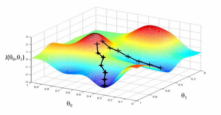
  A visualization of learning rate during stochastic gradient descent, showing two possible solutions for a minimized cost function. You can also imagine a hyperplane being created at each point that directs the algorithm which way to descend.

• cross-validation: Fundamentally, this is the same concept as in the social sciences, which is an approach to determine how generalizable the estimates in a model are to other samples.  However, in machine learning, the way you approach cross-validation is a bit different, which is possible due to the large samples commonly found here, especially those associated with “big data.”
• big data: Such a general and overused term that it now has near-zero value.  It used to mean, “datasets that cannot be analyzed with traditional methods for any of a variety of reasons,” but the datasets that applied to even 3 years ago no longer fall within that definition.  Unless you’re at the point where the data you’re collecting literally cannot be viewed in SPSS (for whatever reason), you probably don’t have big data.
• 10-fold cross-validation: This is a very common type of cross-validation in machine learning in which a dataset is divided into 10 parts (i.e., folds), then a machine learning algorithm is applied to create your specified predictive model 10 times: using the data in 9 folds to predict the 10th, repeated for all 10.  This procedure creates a distribution of R^2s and mean square error terms.  The reason you might want to do that is that by creating a shared output metric across all of the algorithms you try, you can compare the distributions of these statistics across different algorithms in a meaningful way.  For example, if you tried to predict y from 200 ‘x’ variables and found equal R^2s for two different machine learning algorithms (each already tested to determine it is using ideal hyperparameters given the dataset) yet the distribution of mean square errors across folds was wider for algorithm #1 than #2, you’d probably trust algorithm #2 to replicate out of sample more than you trust algorithm #1.

There are so many new terms in machine learning, but I hope that gives you some understanding of the most basic. As you can see, in many cases, the concepts are just a relatively small twist on other concepts you already know. At the very least, you need to be able to hold an intelligent conversation with the data scientists on your team, and hopefully this will help with that. If you have any requests or your own definitions for terms, please share them!